The Example Workbook
Extract and open the workbook linked to in the Files Needed
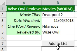
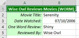
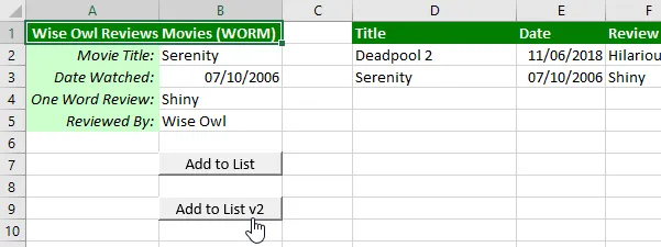
section above. The worksheet asks you to enter a review for a movie:

You can add a review of a film you have seen here.
We want to create a procedure which we can attach to the button which will
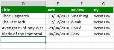
add your review to the list of reviews on the right:

Clicking the button should add your review to the bottom of the existing list.
Selecting the Next Blank Row
One way to complete this task is to select the next blank cell in column
D and use this as the starting point to copy the data you have
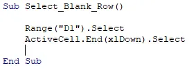
entered. In the VBE, insert a new module and create a subroutine which
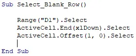
begins by selecting cell D1:

Range
D1 is the cell at the top of the first column of the table.
To find the last populated cell in the column, we can use the End
property moving in the downwards direction. Add an instruction to do this:

Set the
Direction parameter of the
End property to xlDown.
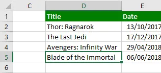
Running the subroutine at this point will select cell D5:

D5 is the cell immediately above the next blank cell in
the column.
Having reached this point, we can use the Offset property to
move one cell down to reach the next blank one. Add an instruction to do
this:

Set the
RowOffset parameter to 1 and the
ColumnOffset parameter to
0.
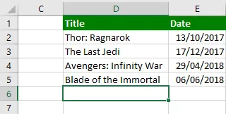
Running the subroutine at this point will select cell D6:

You'll end up in this cell if you run the subroutine.
Combining End and Offset
Rather than writing three separate instructions to reach the next blank cell,
you can combine the End and Offset properties
in a single instruction. Edit your code to refer to cell D1:

Get rid of everything except the reference to cell
D1.
Now apply the End property to the range you have referenced:

Apply the
End property and specify the
xlDown direction.
Now apply the Offset property to the range returned by the
End property:

We're still offsetting
1 row down and 0 columns.
Finally, you can apply the Select method to the range returned
by the Offset property:

This single instruction has the same effect as the three instructions it replaces.
You can run the subroutine to check that it selects the appropriate cell.
Copying Values into the Selected Row
Now that we've reached the next blank row, we can transfer the values you
have entered into the appropriate cells:

We'll start by copying the value of cell
B2 into the cell we have just selected.
We can use the ActiveCell property to refer to the selected
cell. Rather than copying and pasting, we'll simply change the value of
this cell:

Make the value of the
ActiveCell equal to the value of cell B2.
Next, we want to change the value of the cell one column to the right of the
active cell to equal the value of cell B3. Start by using
the Offset property to refer to the value of the cell one
column to the right of the currently selected cell:

Set the
RowOffset to 0 and the ColumnOffset to
1.
You can now make the value of the referenced cell equal to the value of cell
B3:

Assign the value of cell
B3 to the referenced cell.
You can use the same technique to populate the final two columns of the table.
You'll need to increase the number of the ColumnOffset
parameter as you work along the row:

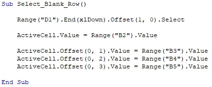
The final subroutine should look like this.
Testing
the Procedure
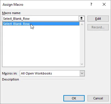
To test the subroutine, assign it to the button on the worksheet:

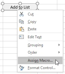
Right-click the button and choose
Assign Macro...
Select the subroutine you have written:

Double-click the name of the subroutine you have written.
Click on any cell in the worksheet and then click the button to check that it
works:

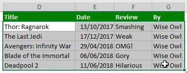
After clicking the button once you should see the details are copied to the bottom of the list.
What Happens When the List is Empty
The technique we have used here relies on the list containing at least one
row of data. If the list is empty, the procedure will fail. Test
this by deleting the existing data from the list:

Select and delete the cells containing the data in the table (or just move the data somewhere else if you want to keep it).
Leave the column headings in place.
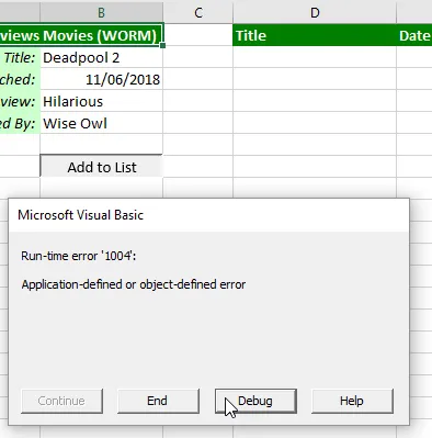
Click the button on the worksheet (or just run the subroutine from the VBE):

Running the subroutine causes a run-time error. You can click Debug to see the line which has caused this.
If you click Debug you'll see which line of code
has caused the run-time error:

The first line of the procedure causes the problem.
When the list of data is empty, the End property refers to the cell at the
bottom of column D, cell D1048576. The
Offset property then tries to refer to the cell below it but, because
this cell doesn't exist, the Select method fails.
One way to resolve this is to start at the bottom of the column and go
upwards instead. Start by changing the address of the cell you refer to in
the first instruction:

Refer to cell
D1048576. This is the last cell in column
D.
Next, change the direction of the End property to move upwards
instead of downwards:

Change the direction to
xlUp.
Try running the subroutine again and check that the results appear in the
correct place:

This version of the procedure works whether or not the list already contains data.


