Having fun with spill arrays (dynamic arrays) in Excel
My love for Excel's new(ish) spill arrays has blossomed since their release.
To share this love, I thought I'd give four case studies to show how you can
use them to add elegance and simplicity to your Excel workbooks.
If you're not sure about any of the concepts behind (or syntax of) any of the
dynamic array functions used in the case studies below, have a look at my
earlier blog about the structure and use of dynamic array
functions.
Example 1 of 4 - Creating Month Headers
A common modelling requirement is to create headers for the coming 12 months:

These headers start at the end of the current month (at the time of writing), and run for 12 months. The second row shows the month names.
Here's the formula for the first row:

See below for an explanation of what this does.
Here's how this formula works:
|
Function |
Explanation of use |
|
TODAY |
Returns today's date (2nd September 2022 at the time of writing). |
|
EOMONTH |
Returns the end of the month N days forward from the current month (so if
N is 0, for example, this would just give the end of the current month, or
30/09/2022). |
|
SEQUENCE |
Creates a sequence of integers occupying 1 row and 12 columns, beginning at 0
and going up by 1 each time. |
Finally, you can derive the month names by suffixing a #
character to a cell reference to refer to the whole spilled array instead:

This function takes each date in the spilled array and picks out the month name.
Example 2 of 4 - mortgage affordability scenarios
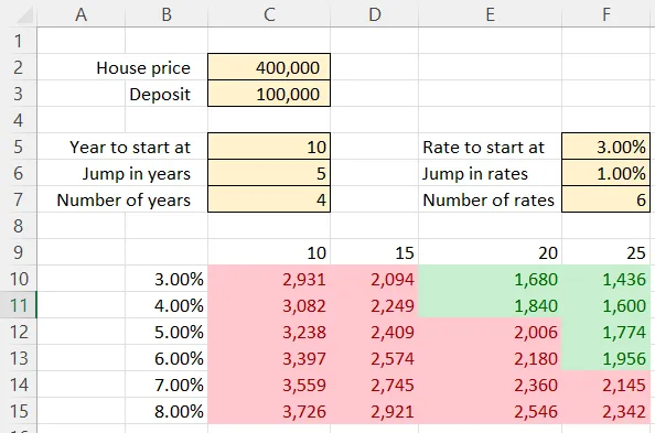
This example produces a two-day data table showing the extent to which you
can afford a mortgage based on different terms and interest rates:

The table assumes a repayment mortgage. Conditional formatting has been applied to show mortgages that you can afford (anything up to £2,000 a month, say).
The yellow(ish) cells at the top are inputs. So you can specify:
- The price of the house you want to buy, and how much deposit
you can put down.
- The parameters for how many years you display along the top,
and what the gap is between each pair of years.
- The parameters for the interest rates down the left-hand
side, including where they start and how many rates there are.
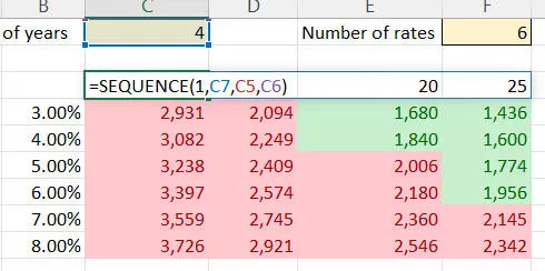
The row headers are given by this SEQUENCE function:

The sequence gives one row and N columns (where N is the number held in cell
C7), starts at the number held in C5 and jumps by the number held in
C6 for each new term.
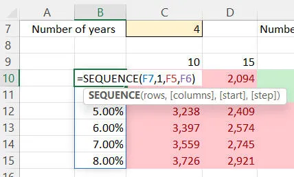
Here are the
column headers:

The interest rates occupy
F7 rows and 1 column, start at F5 and jump by
F6 years for each new term.
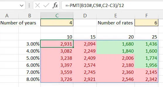
Finally, here is the formula filling the table of data:

The
PMT function gives the total payment made each year as an outgoing. We reverse the sign and divide by 12 to get the monthly payment.
The arguments to the PMT function as used above are:
|
Argument
|
Meaning |
As used above |
|
1 |
Interest rate |
The spilled array containing the column of interest rates
to the
left of the grid. |
|
2 |
Term in years |
The spilled array containing the row of terms in years
above the grid. |
|
3 |
Loan to repay |
The difference between the house price and the deposit put down. |
Notice that there's no need for any absolute cell references using %
signs: Excel knows the dimensions of each spilled array, and automatically
returns a grid with the chosen number of rows and columns.
Example 3 of 4 - constructing a league table
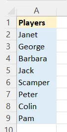
This example involves taking a list of players in a league:

To make life easier I've given the list of players in blue the range name
Players.
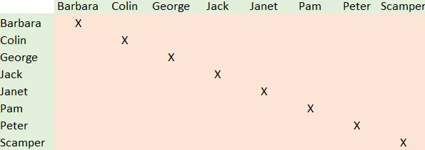
From this we'll construct this league:

The players' names are in alphabetical order.
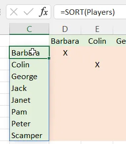
It's easy to get the names on the left:

We sort the players alphabetically by name.
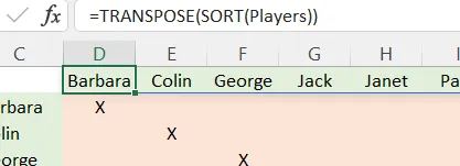
You can get the top row of names by transposing the names:

We sort the names and then turn the column into a row by transposing them.
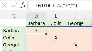
Finally, you can put in an X in the cells whose games can't
happen:

Again, notice that the # character refers to the spilled array (and that we don't need any $ signs or absolute cell references).
Example 4 of 4 - filtering tables of volunteers
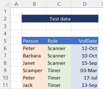
I got a bit carried away with this one. The aim is to take a table of
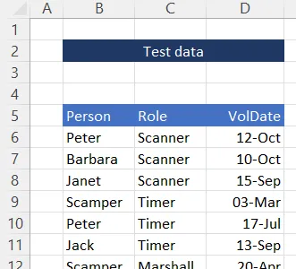
Park Run volunteers:

I've got 30 volunteers in this table. I originally used the dynamic array function
RANDARRAY to fill the table, but then discovered that because this is what's called a
volatile function Excel generates spill errors further down the line
(since it can't predict the number of rows and columns returned always).
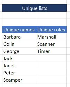
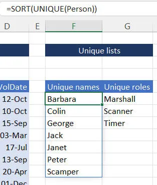
From this we'll derive unique sorted lists of names and roles:

Intermediate tables of names and roles (you could always hide these columns).
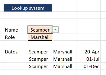
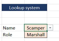
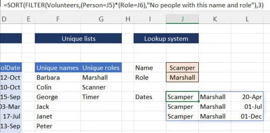
We'll then use these to create a lookup system:

The list of dates when Scamper has volunteered to be a marshall.
I started this by creating 3 range names called Person,
Role and VolDate:

You don't have to do this - you could just use
the cell references instead.
I then created the sorted list of unique names and roles:

The formula for the unique list of people's names, sorted alphabetically (the role formula would be similar, but using the
Role range name).
You can then apply data validation to the following two cells to restrict a user's
choices:

A user should only be able to choose an existing name and role.
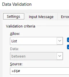
Here's the data validation setting for the name, for example:

You can only choose one of the sorted list of unique names.
You can now apply a filter to the table of data to return those volunteers
having the right name and role:

The range name called
Volunteers refers to the original table of data (A6:D35). Two conditions must be true: the person must match the one chosen above in cell
J5 and the role must match the one chosen above in cell
J6. If there aren't any such people, you get a suitable message to this effect.
Finally, for fun, I thought I'd list out the dates chosen:

The concatenated list of dates from the list of volunteers meeting the filter criteria.
Here's the formula for this:
=TEXTJOIN(", ",TRUE,TEXT(INDEX(J8#,,3),"dddd dd mmmm yyyy"))
The arguments to the TEXTJOIN function are:
|
Argument |
Use |
|
1 |
The delimiter (separator) to use |
|
2 |
Whether to include blank values (there can't be any, so
this is irrelevant) |
|
3 |
A range containing a list of values to concatenate.
Here this uses the INDEX function with no row argument to
return the third column of the returned spilled array, and uses the TEXT
function to format this suitably. |
You can see
all of the examples in this blog (and more) in action in this workbook.


